PAA 2024 Supplemental Poster Tables and Figures
Important Terms, Concepts, and Notes
Spatial Assimilation, coined by Doug Massey, refers to the process whereby a group attains residential propinquity with members of a host society.
Place Stratification, a theory that emerged as a result of political economy’s influence in the late 80s, refers to the persistence of prejudice and discrimination that act to constrain the residential mobility options of disadvantaged groups.
Public Use Microdata Areas (PUMAs), the smallest, publicly-available ecological unit from the Integrated Public Use Microdata Series (IPUMS) U.S.A. database, and it contains at least 100,000 individuals.
Latent Class Analysis, a method that allows for the dependent variable to take on a more robust set of variables to characterize qualitatively different subgroups, and at the same time runs an underlying multinomial logistic regression model to explore more complex relationships between latent outcomes and predictor variables. In this case, I use a 4-class model.
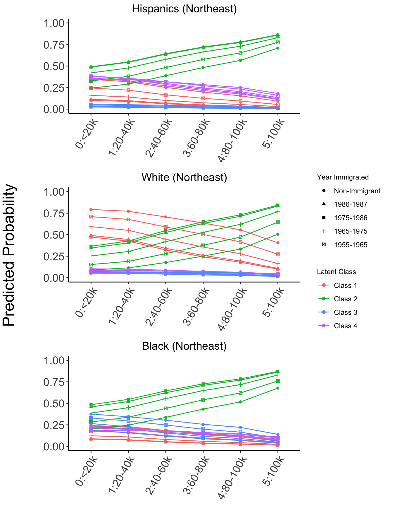
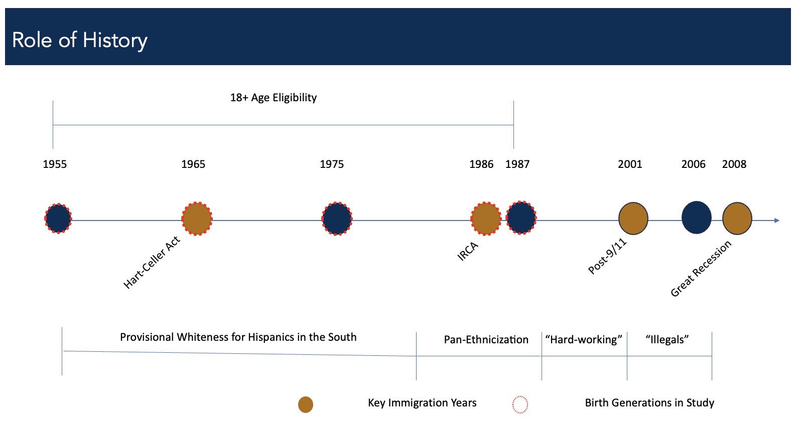
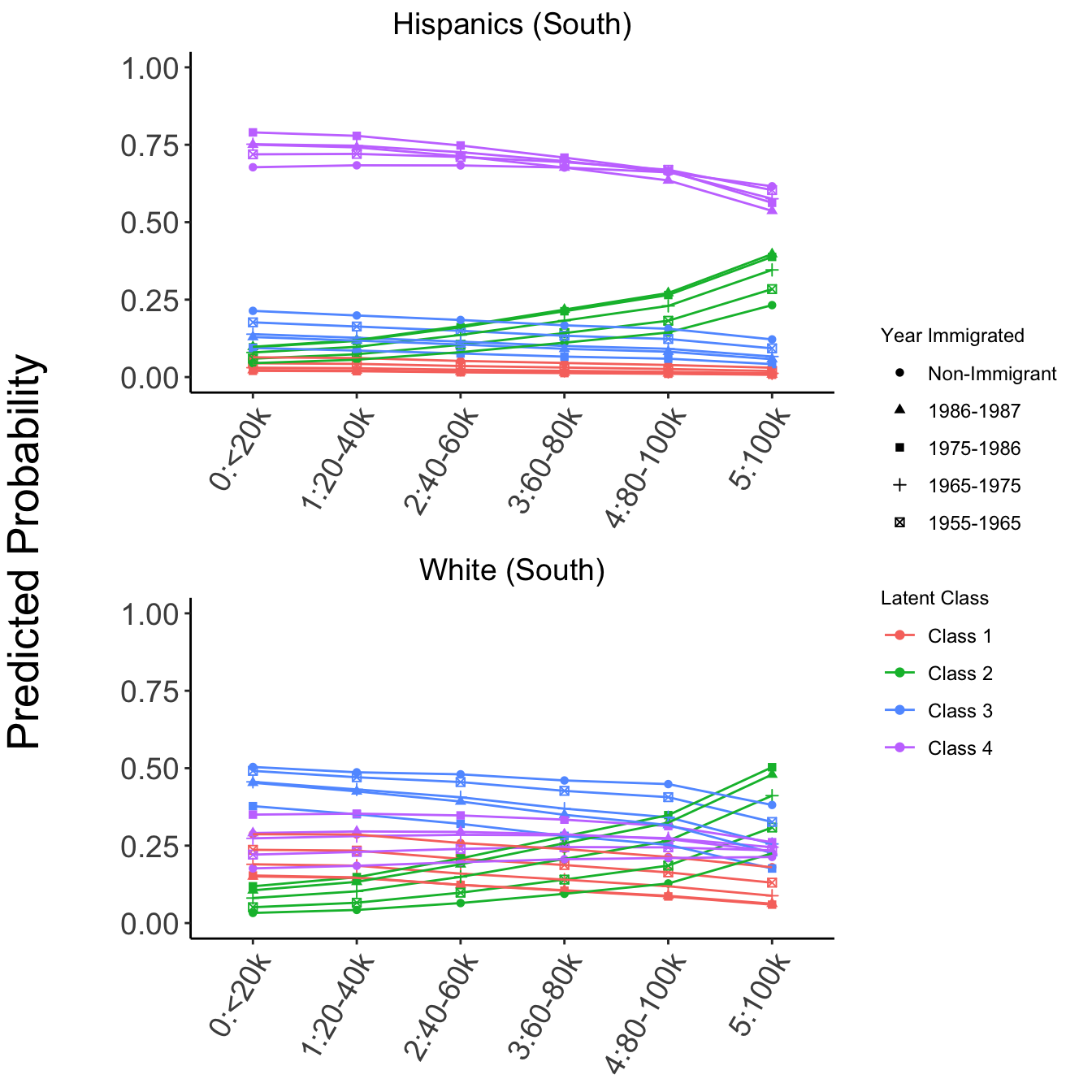
A note on the year immigrated variable: Figure 3 breaks things down by year immigrated. Why is this important? For many reasons! Years 1955-1965 was the decade following the 1954 Operation Wetback, which was a federal government-sponsored initiative that began to crack down on illegal immigration. Then, in 1965, the Hart-Celler Act (or otherwise known as the Immigration and Nationality Act of 1965) opened up new pathways for immigrants from historically underrepresented countries, while at the same time legalizing and institutionalizing quotas. It wasn’t until the next big immigration act, the 1986 IRCA (also known as the Immigration Reform and Control Act), that changed a lot of things: it regulated the employment of undocumented immigrants, increased border militarization at the U.S.-Mexico border, and allocated funds for detention centers, surveillance hardware, police patrolling, and fencing, all while labor-demand in the South was rising rapidly. Hence, these years are explored to determine any significant outcomes between ethnoracial groups.
Visualizations on Poster
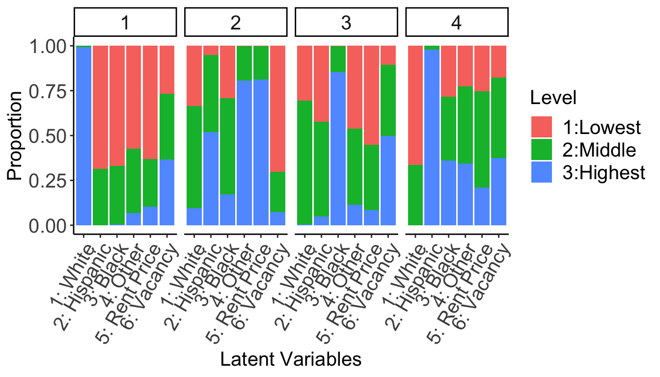
- Figure 1: Latent Class Ideal Area-Type Makeup.
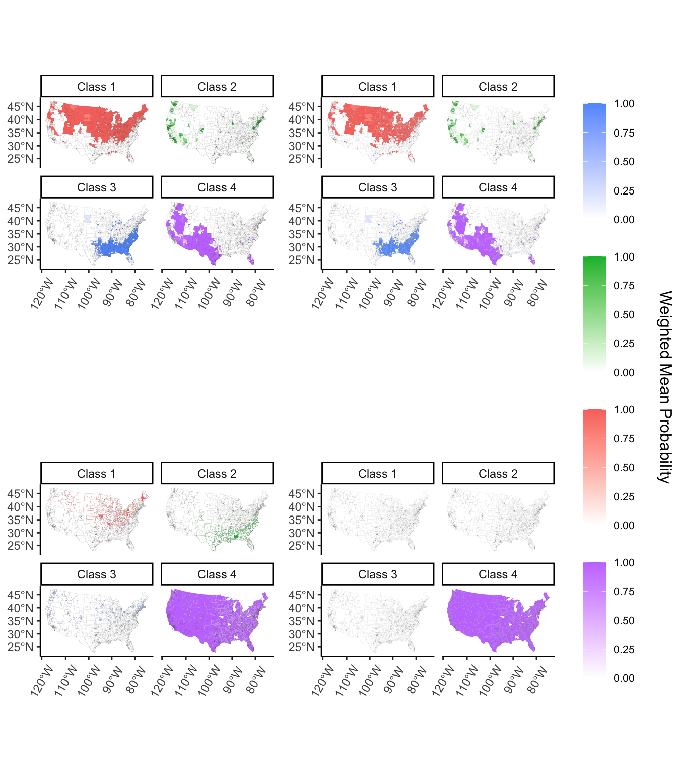
- Figure 2: Mapping Predicted Outcomes With and Without Regional Variation.
- Figure 3: Comparing White and Hispanic Southerners.
Additional Tables and Figures
- Observed Sample Statistics and Proportions by Region.
| Variable | Levels | Northeast | Midwest | South | West | p |
|---|---|---|---|---|---|---|
| Latent Variables | ||||||
| White Prop | [0.00142,0.611) | 20995 (17.3) | 16339 (9.4) | 83135 (32.9) | 62264 (43.3) | <0.001 |
| [0.61055,0.850) | 32242 (26.5) | 34238 (19.8) | 121962 (48.2) | 54890 (38.1) | ||
| [0.85027,0.991] | 68337 (56.2) | 122628 (70.8) | 47814 (18.9) | 26752 (18.6) | ||
| Hispanic Prop | [0.0000,0.0319) | 53900 (44.3) | 103840 (60.0) | 80464 (31.8) | 5658 (3.9) | <0.001 |
| [0.0319,0.1257) | 42350 (34.8) | 57232 (33.0) | 91177 (36.1) | 43894 (30.5) | ||
| [0.1257,0.9796] | 25324 (20.8) | 12133 (7.0) | 81270 (32.1) | 94354 (65.6) | ||
| Black Prop | [0.0000,0.0281) | 55807 (45.9) | 90620 (52.3) | 27855 (11.0) | 77740 (54.0) | <0.001 |
| [0.0281,0.1186) | 40965 (33.7) | 54816 (31.6) | 88724 (35.1) | 53285 (37.0) | ||
| [0.1186,0.9838] | 24802 (20.4) | 27769 (16.0) | 136332 (53.9) | 12881 (9.0) | ||
| Other Prop | [0.0000,0.0171) | 39803 (32.7) | 82974 (47.9) | 107363 (42.5) | 9391 (6.5) | <0.001 |
| [0.0171,0.0453) | 40969 (33.7) | 64004 (37.0) | 93184 (36.8) | 39122 (27.2) | ||
| [0.0453,0.7829] | 40802 (33.6) | 26227 (15.1) | 52364 (20.7) | 95393 (66.3) | ||
| Median Rent | [200, 505) | 33314 (27.4) | 102208 (59.0) | 115468 (45.7) | 19623 (13.6) | <0.001 |
| [505, 705) | 31512 (25.9) | 52317 (30.2) | 87516 (34.6) | 46290 (32.2) | ||
| [705,1700] | 56748 (46.7) | 18680 (10.8) | 49927 (19.7) | 77993 (54.2) | ||
| Vacant Prop | [ 0.666, 6.66) | 54944 (45.2) | 50316 (29.0) | 47829 (18.9) | 72097 (50.1) | <0.001 |
| [ 6.663,11.41) | 34347 (28.3) | 72432 (41.8) | 94371 (37.3) | 41900 (29.1) | ||
| [11.410,56.39] | 32283 (26.6) | 50457 (29.1) | 110711 (43.8) | 29909 (20.8) | ||
| Predictor Variables | ||||||
| Mover Status | Moved | 15137 (12.5) | 25096 (14.5) | 44817 (17.7) | 26618 (18.5) | <0.001 |
| Did not Move | 106437 (87.5) | 148109 (85.5) | 208094 (82.3) | 117288 (81.5) | ||
| Ethnoracial Identity | Black | 8338 (6.9) | 9433 (5.4) | 35049 (13.9) | 4906 (3.4) | <0.001 |
| Hispanic | 9795 (8.1) | 7556 (4.4) | 32700 (12.9) | 36885 (25.6) | ||
| White | 103441 (85.1) | 156216 (90.2) | 185162 (73.2) | 102115 (71.0) | ||
| Birth Cohort | 1955-1965 Cohort | 55064 (45.3) | 74877 (43.2) | 103773 (41.0) | 58682 (40.8) | <0.001 |
| 1965-1975 Cohort | 43047 (35.4) | 57553 (33.2) | 87124 (34.4) | 49527 (34.4) | ||
| 1975-1986 Cohort | 22773 (18.7) | 39092 (22.6) | 59121 (23.4) | 34084 (23.7) | ||
| 1986-1987 Cohort | 690 (0.6) | 1683 (1.0) | 2893 (1.1) | 1613 (1.1) | ||
| Immigrant Cohort | 1955-1965 IM | 759 (0.6) | 540 (0.3) | 1496 (0.6) | 1125 (0.8) | <0.001 |
| 1965-1975 IM | 1766 (1.5) | 948 (0.5) | 2811 (1.1) | 2715 (1.9) | ||
| 1975-1986 IM | 3502 (2.9) | 1796 (1.0) | 6645 (2.6) | 8632 (6.0) | ||
| 1986-1987 IM | 11127 (9.2) | 6295 (3.6) | 21629 (8.6) | 19352 (13.4) | ||
| Non-Immigrant | 104420 (85.9) | 163626 (94.5) | 220330 (87.1) | 112082 (77.9) | ||
| Education (Years) | Mean (SD) | 13.9 (2.6) | 13.5 (2.3) | 13.3 (2.7) | 13.3 (3.0) | <0.001 |
| Household Income | [<20K) | 9705 (8.0) | 16339 (9.4) | 29424 (11.6) | 13393 (9.3) | <0.001 |
| [20k-40k) | 17708 (14.6) | 30652 (17.7) | 48785 (19.3) | 25680 (17.8) | ||
| [40k-60k) | 21424 (17.6) | 36410 (21.0) | 50175 (19.8) | 26746 (18.6) | ||
| [60k-80k) | 20315 (16.7) | 32735 (18.9) | 40680 (16.1) | 22951 (15.9) | ||
| [80k-100k) | 15555 (12.8) | 22060 (12.7) | 28771 (11.4) | 16894 (11.7) | ||
| [100k+] | 36867 (30.3) | 35009 (20.2) | 55076 (21.8) | 38242 (26.6) | ||
| Renter Status | Rented | 34124 (28.1) | 38279 (22.1) | 72825 (28.8) | 51359 (35.7) | <0.001 |
| Not Rented | 87450 (71.9) | 134926 (77.9) | 180086 (71.2) | 92547 (64.3) | ||
| Self-Employed Status | Self-Employed | 15083 (12.4) | 20186 (11.7) | 31398 (12.4) | 21167 (14.7) | <0.001 |
| Not Self-Employed | 106491 (87.6) | 153019 (88.3) | 221513 (87.6) | 122739 (85.3) | ||
| Married-Couple Status | Married-Couple Household | 85837 (70.6) | 124899 (72.1) | 176653 (69.8) | 100091 (69.6) | <0.001 |
| Non-Married-Couple Household | 35737 (29.4) | 48306 (27.9) | 76258 (30.2) | 43815 (30.4) | ||
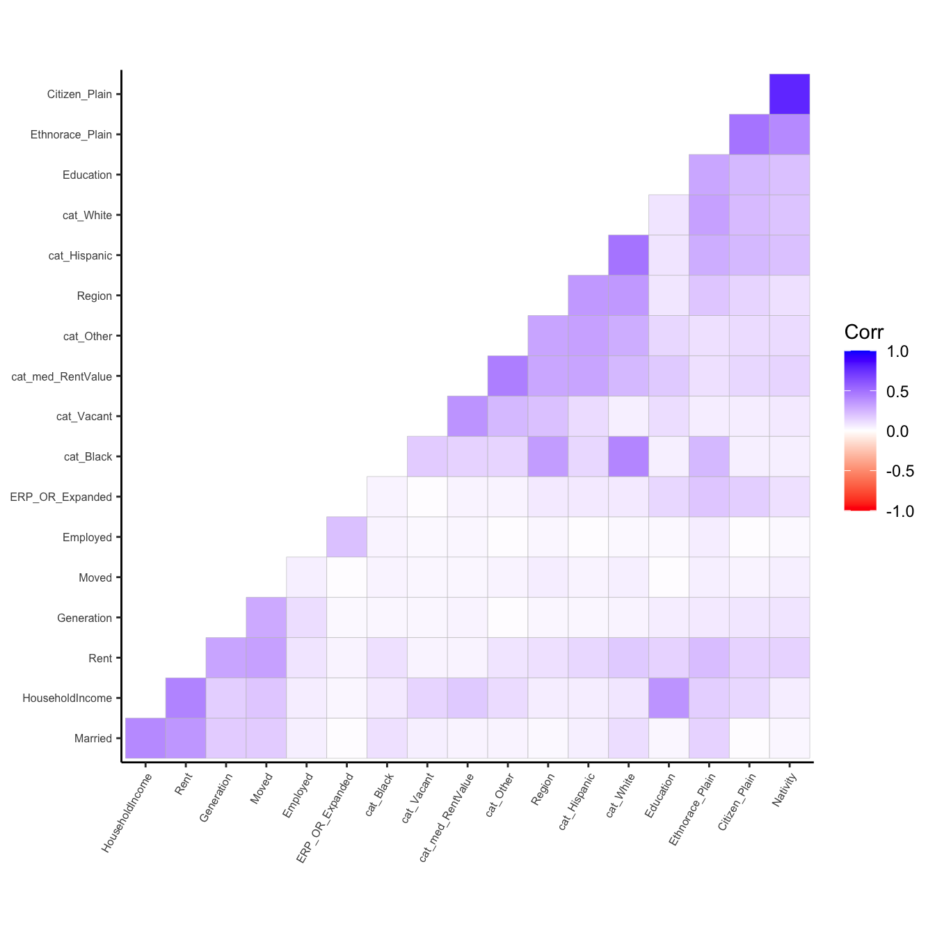
- Correlation Plot Displaying Pairwise Associations of Chi-Squared Tests Between Categorical Variables, Pearson Correlation Tests Between Numeric Variables, and ANOVA Tests Between Categorical and Numerical Variables with Association Cutoffs at 0.7.
- Model Output for Both Models.
| Intercept | -1.2 (0.03) | -3.4 (0.037) | -3.3 (0.028) | -4.3 (0.033) | -2.7 (0.031) | -3.6 (0.035) |
| Mover Status (Baseline: Did not Move) | ||||||
| Moved | 0.14 (0.013) | 0.16 (0.015) | 0.18 (0.012) | -0.0053 (0.013) | -0.024 (0.012) | 0.039 (0.013) |
| Ethnoracial Status (Baseline: White) | ||||||
| Black | 3.2 (0.026) | 0.56 (0.038) | 2.2 (0.027) | 2 (0.025) | 2.9 (0.02) | 2.6 (0.023) |
| Hispanic | -14 (3.3e-15) | 4.1 (3.5e-07) | 21 (6e-07) | 1.8 (0.021) | 0.64 (0.025) | 2.8 (0.02) |
| Birth Cohort (Baseline: 1955-1965 Cohort) | ||||||
| 1965-1975 | 0.035 (0.01) | 0.015 (0.011) | 0.018 (0.0089) | 0.04 (0.0099) | 0.014 (0.0096) | -0.017 (0.011) |
| 1975-1986 | 0.14 (0.012) | -0.0072 (0.014) | 0.046 (0.011) | 0.026 (0.013) | 0.14 (0.011) | 0.035 (0.013) |
| 1986-1987 | 2.1 (1.6e-06) | 19 (0.018) | 18 (0.018) | -0.083 (0.051) | 0.076 (0.039) | -0.086 (0.045) |
| Immigrant Cohort (Baseline: Non-Immigrant) | ||||||
| 1955-1965 | 0.44 (0.077) | 0.69 (0.075) | 1.1 (0.06) | 0.64 (0.054) | 0.17 (0.062) | 0.42 (0.061) |
| 1965-1975 | 0.44 (0.073) | 1.1 (0.069) | 1.6 (0.057) | 1.3 (0.041) | 0.31 (0.052) | 0.85 (0.046) |
| 1975-1986 | 0.3 (0.074) | 1.3 (0.072) | 2.3 (0.059) | 1.9 (0.033) | 0.34 (0.042) | 1.3 (0.035) |
| 1986-1987 | 0.58 (0.052) | 1.9 (0.049) | 2.8 (0.043) | 1.8 (0.02) | 0.54 (0.025) | 1.1 (0.022) |
| Educ | 0.051 (0.0021) | 0.16 (0.0023) | 0.19 (0.0018) | 0.17 (0.0018) | 0.033 (0.0019) | 0.068 (0.002) |
| Household Income (Baseline: <20k) | ||||||
| 20-40k | -0.038 (0.016) | 0.24 (0.023) | 0.27 (0.016) | 0.26 (0.021) | -0.032 (0.016) | 0.05 (0.018) |
| 40-60k | 0.017 (0.017) | 0.58 (0.023) | 0.71 (0.016) | 0.78 (0.021) | 0.056 (0.016) | 0.21 (0.019) |
| 60-80k | 0.046 (0.018) | 0.91 (0.024) | 1.1 (0.017) | 1.2 (0.021) | 0.092 (0.017) | 0.34 (0.02) |
| 80-100k | 0.23 (0.02) | 1.3 (0.025) | 1.6 (0.019) | 1.7 (0.022) | 0.18 (0.019) | 0.47 (0.022) |
| 100k+ | 0.43 (0.02) | 1.9 (0.024) | 2.4 (0.018) | 2.4 (0.021) | 0.19 (0.018) | 0.65 (0.021) |
| Renting Unit? (Baseline: Not Renting) | ||||||
| Yes | 0.19 (0.012) | 0.25 (0.014) | 0.88 (0.011) | 0.77 (0.012) | 0.26 (0.011) | 0.45 (0.013) |
| Self-Employed? (Baseline: Not Self-Employed) | ||||||
| Yes | -0.023 (0.013) | 0.029 (0.014) | 0.17 (0.011) | -0.012 (0.013) | -0.073 (0.013) | 0.051 (0.014) |
| Married-Couple? (Baseline: Non-Married-Couple) | ||||||
| Yes | -0.27 (0.011) | -0.44 (0.013) | -0.74 (0.0099) | -0.7 (0.011) | -0.38 (0.01) | -0.53 (0.012) |
| Region (Baseline: Northeast) | ||||||
| Midwest | -1.3 (0.013) | 0.61 (0.016) | -1 (0.024) | |||
| South | -0.00012 (0.013) | 3 (0.015) | 2.3 (0.018) | |||
| West | 2 (0.013) | -9.9 (2.3e-06) | 2.6 (0.02) | |||
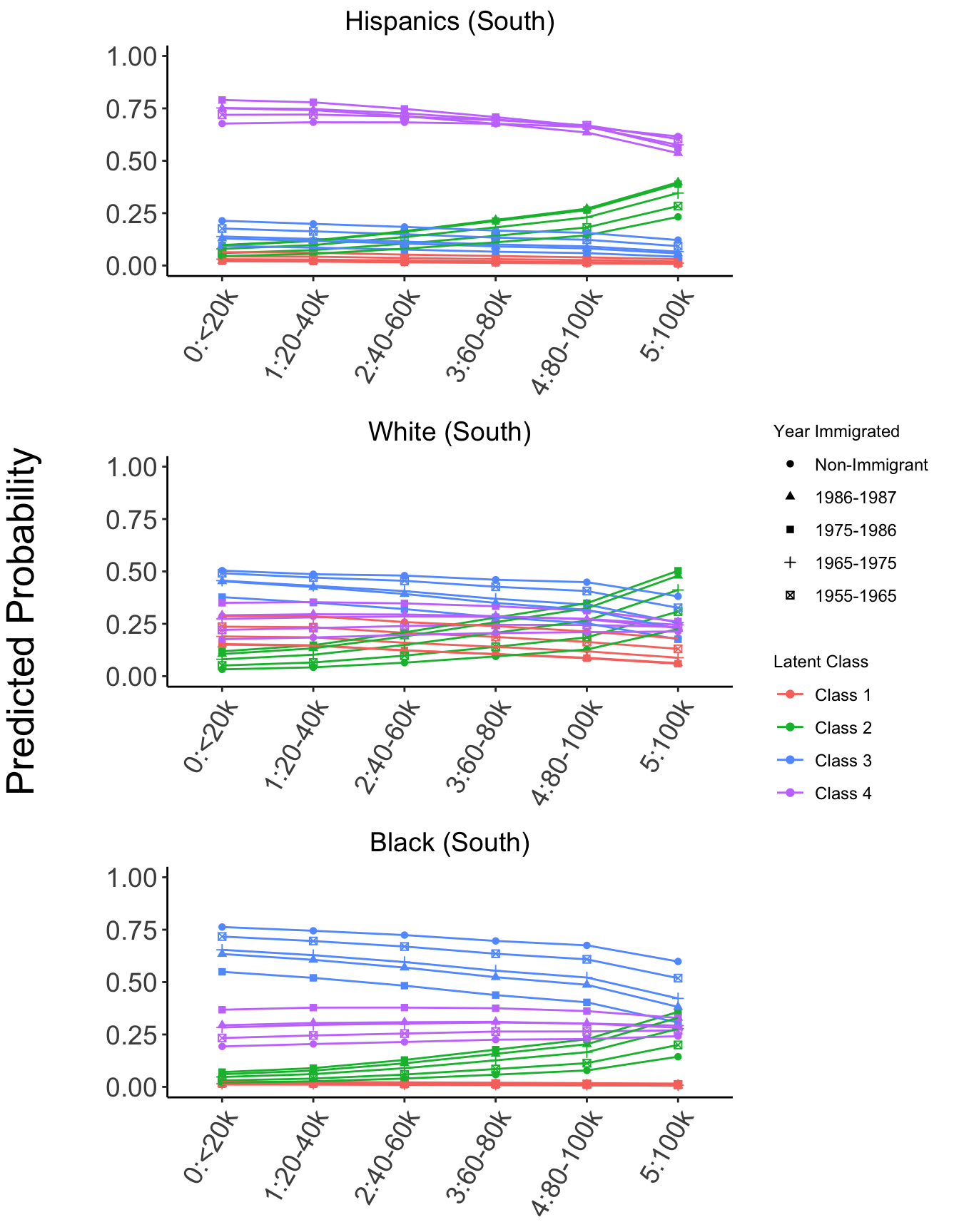
- Same as Figure 3, except comparing White, Black, and Hispanic Southerners.
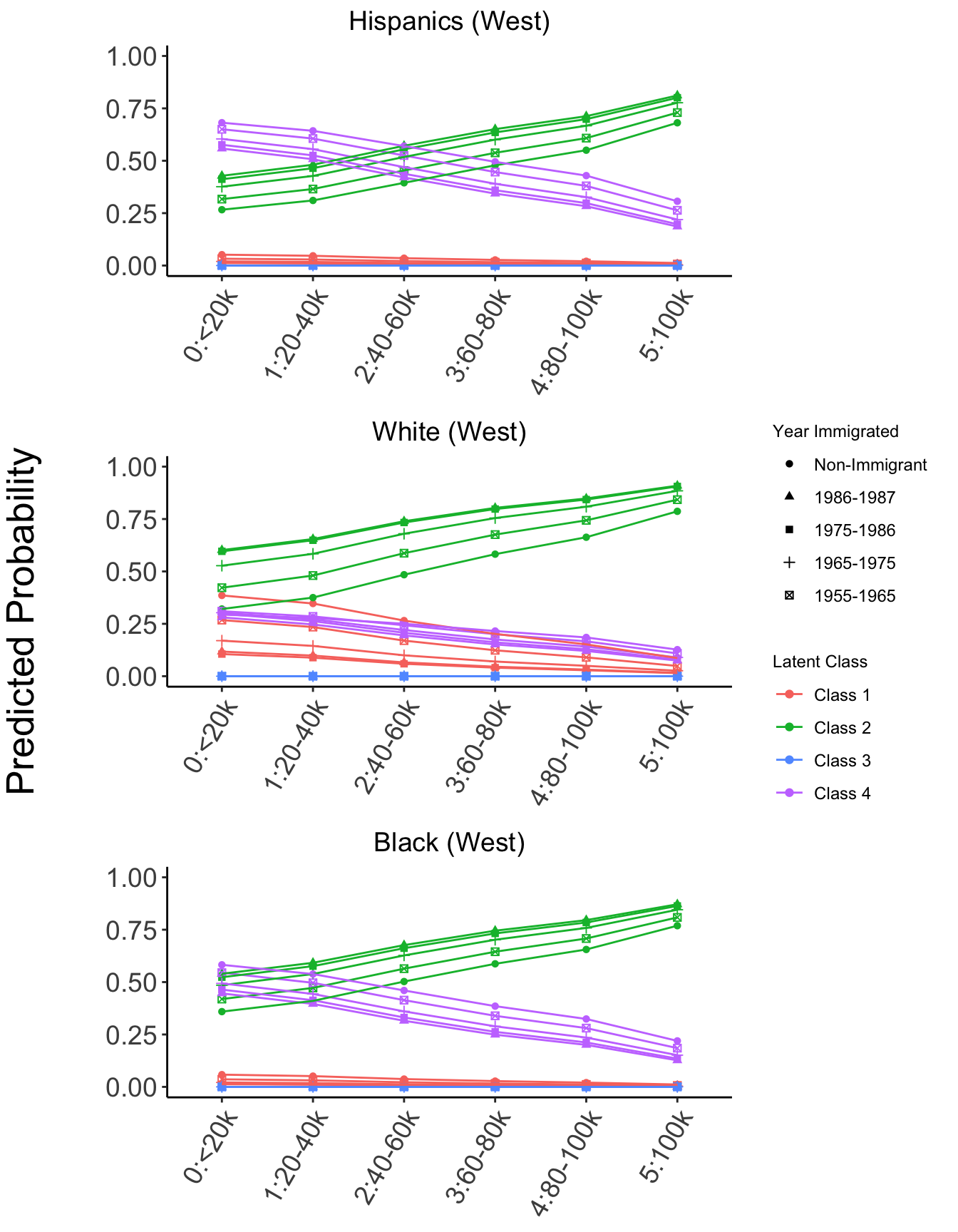
- Same as last figure except comparing White, Black, and Hispanic Westerners.
- And for Northeasterners!